LINEAR PROGRAMMING : A WORD PROBLEM WITH FOUR VARIABLES ----- BY. MWL. JAPHET MASATU

Linear Programming:
  A Word Problem with Four Variables .
Sections: Optimizing linear systems, Setting up word problems

---

INTRODUCTION:

• A building supply has two locations in town. The office receives orders from two customers, each requiring 3/4-inch plywood. Customer A needs fifty sheets and Customer B needs seventy sheets.
The warehouse on the east side of town has eighty sheets in stock; the west-side warehouse has forty-five sheets in stock. Delivery costs per sheet are as follows: $0.50 from the eastern warehouse to Customer A, $0.60 from the eastern warehouse to Customer B, $0.40 from the western warehouse to Customer A, and $0.55 from the western warehouse to Customer B.
Find the shipping arrangement which minimizes costs.
Hmm... I've got four things to consider:

east warehouse to Customer A
east warehouse to Customer B
west warehouse to Customer A
west warehouse to Customer B
But I only have two variables. How can I handle this?
The variables obviously need to stand for the number of sheets being shipped, but I have four different sets of sheets. This calls for subscripts and explicit labelling:

shipped from east warehouse to Customer A: A_e
shipped from west warehouse to Customer A: A_w
shipped from east warehouse to Customer B: B_e
shipped from west warehouse to Customer B: B_w
Since Customer A wants 50 sheets and Customer B wants 70 sheets, then:

A_e + A_w = 50, so A_w = 50 – A_e   (I'll call this Equation I)
B_e + B_w = 70, so B_w = 70 – B_e   (I'll call this Equation II)
Since the eastern warehouse can ship no more than eighty sheets and the western warehouse can ship no more than forty-five sheets, then:

0 < A_e + B_e < 80
0 < A_w + B_w < 45
And the optimization equation will be the shipping cost:

C = 0.5A_e + 0.6B_e + 0.4Aw + 0.55Bw
Where does this leave me? The equations (labelled as Equations I and II above) allow me to substitute and get rid of two of the variables in the second inequality above, so:

0 < A_e + B_e < 80
0 < (50 – A_e) + (70 – B_e) < 45
Simplifying the second inequality above gives me the new system:

0 < A_e + B_e < 80
0 < 120 – A_e – B_e < 45
Multiplying through by –1 (thereby flipping the inequality signs) and adding 120 to all three "sides" of the second inequality, I get the new system:

0 < A_e + B_e < 80
120 > A_e + B_e > 75
Since A_e + B_e is no less than 75 and is no more than 80, then these two inequalities reduce to one:


75 < A_e + B_e < 80
I can also simplify the optimization equation:

C = 0.5A_e + 0.6B_e + 0.4Aw + 0.55Bw
    = 0.5A_e + 0.6B_e + 0.4(50 – A_e) + 0.55(70 – B_e)
    = 0.1A_e + 0.05B_e + 58.50
Due to the size of the orders, I have:

0 < A_e < 50
0 < B_e < 70
Since I have only two variables now, and since I'll be graphing with x and y, I'll rename the variables:   Copyright © Elizabeth Stapel 2006-2011 All Rights Reserved

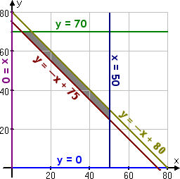
x = A_e
y = B_e
Then entire system is as follows:


Minimize C = 0.1x + 0.05y + 58.50, subject to the following:
x > 0 y > 0 y > –x + 75	x < 50 y < 70 y < –x + 80

The feasibility region graphs as:

When you test the corner points, (5, 70), (10, 70), (50, 30), and (50, 25), you should get the minimum cost when you ship as follows:
  5 sheets from the eastern warehouse to Customer A70 sheets from the eastern warehouse to Customer B45 sheets from the western warehouse to Customer A
  0 sheets from the western warehouse to Customer B